Correlation and Regression

I greet you this day,

First: Read the stories. (Yes, I tell stories too. ☺)
The stories will introduce you to the topic, while making you smile/laugh at the same time.
Second: Review the Notes.
Third: View the Videos.
Fourth: Solve the questions/solved examples.
Fifth: Check your solutions with my thoroughly-explained solved examples.
Sixth: Check your answers with the calculators.

I wrote the codes for the calculators using Javascript, a client-side scripting language.
Please use the latest Internet browsers. The calculators should work.
Comments, ideas, areas of improvement, questions, and constructive criticisms are welcome. You may contact me.
Thank you for visiting.
Samuel Chukwuemeka (Samdom For Peace) B.Eng., A.A.T, M.Ed., M.S

Objectives

Students will:

(1.) Differentiate between association and causation.
(2.) Discuss correlation.
(3.) Draw scatter diagrams manually.
(4.) Draw scatter diagrams using technology (Texas Instruments (TI) calculator, Pearson Statcrunch, Microsoft Excel, and Google Spreadsheets among others).
(5.) Interpret scatter diagrams.
(6.) Calculate the Pearson's correlation coefficient.
(7.) Interpret the Pearson's correlation coefficient in the context in which it was asked.
(8.) Determine the coefficient of determination.
(9.) Interpret the coefficient of determination.
(10.) Compute residuals.
(11.) Determine the least-squares regression line.
(12.) Determine the correlation coefficient and the least-squares regression line using TI (Texas Instruments) calculators.
(13.) Determine the correlation coefficient and the least-squares regression line using technology (Pearson Statcrunch, Microsoft Excel, and Google Spreadsheets among others).
(14.) Calculate the Spearman's rank correlation coefficient.
(15.) Interpret the Spearman's rank correlation coefficient in the context in which it was asked.
(16.) Calculate the Kendall's rank correlation coefficient.
(17.) Interpret the Kendall's rank correlation coefficient in the context in which it was asked.

Vocabulary Words

relationship, relates, causation, causes, association, is associated with, correlation, correlates with,

Definitions

Linear Correlation is an association between two variables: the predictor variable and the response variable.
The association may or may not be causal.

Causation is an association between two variables in which a change in one variable causes a change in the other variable.
This is otherwise known as cause and effect.

A Linear Correlation is the correlation that shows a linear relationship between the variables.
Linear correlation can be positive linear correlation or negative linear correlation.

A Positive Linear Correlation shows a direct relationship in which an increase in the predictor variable leads to an increase in the response variable, and in which a decrease in the predictor variable leads to a decrease in the response variable.

A Negative Linear Correlation shows an inverse relationship in which an increase in the predictor variable leads to a decrease in the response variable, and in which a decrease in the predictor variable leads to an increase in the response variable.

A Scatter Diagram is a graph that shows the relationship between two variables: the response variable and the predictor variable.

Symbols and Meanings

Symbol	Meaning
$X$	dataset $X$
$x$	$x-values$
$\Sigma$	summation (pronounced as uppercase Sigma)
$\Sigma x$	summation of the $x-values$
$(\Sigma x)^2$	square of the summation of the $x-values$
$\Sigma x^2$	summation of the square of the $x-values$
$\bar{x}$	sample mean of the $x-values$
$s$	sample standard deviation
$s_{x}$	sample standard deviation of the $x-values$
$z_{x}$	$z$ score of an individual sample value $x$
$Y$	dataset $Y$
$y$	$y-values$
$\Sigma y$	summation of the $y-values$
$\Sigma y$	summation of the $y-values$
$(\Sigma y)^2$	square of the summation of the $y-values$
$\Sigma y^2$	summation of the square of the $y-values$
$\bar{y}$	sample mean of the $y-values$
$s_{y}$	sample standard deviation of the $y-values$
$z_{y}$	$z$ score of an individual sample value $y$
$\Sigma xy$	sum of the product of the $x-values$ and the corresponding $y-values$
$n$	sample size
$r$	Pearson's correlation coefficient
$\hat{y}$	predicted values of $y$
$b_0$	$y-intercept$ of the least-squares regression line
$b_1$	slope of the least-squares regression line
$b_2$	slope of the least-squares regression line (For multiple linear regression)
$y - \hat{y}$	residual = observed values of $y$ $-$ predicted values of $y$
$(y - \hat{y})^2$	squared residual
$\Sigma(y - \hat{y})^2$	sum of the squared residual
$R_X$	rank of X-values
$R_Y$	rank of Y-values
$d$	Difference between rank X and rank Y values
$\rho$	Spearman's rank correlation coefficient
$\tau$	Kendall's rank correlation coefficient

Formulas

$ (1.)\;\; \bar{x} = \dfrac{\Sigma x}{n} \\[5ex] (2.)\;\; \bar{y} = \dfrac{\Sigma y}{n} \\[5ex] (3.)\;\; z_{x} = \dfrac{x - \bar{x}}{s_{x}} \\[5ex] (4.)\;\; z_{y} = \dfrac{y - \bar{y}}{s_{y}} \\[5ex] $ First Formula for Standard Deviation

$ (5.)\;\; s_{x} = \sqrt{\dfrac{\Sigma(x - \bar{x})^2}{n - 1}} \\[7ex] (6.)\;\; s_{y} = \sqrt{\dfrac{\Sigma(y - \bar{y})^2}{n - 1}} \\[7ex] $ Second Formula for Standard Deviation

$ (7.)\;\; s_{x} = \sqrt{\dfrac{n(\Sigma x^2) - (\Sigma x)^2}{n(n - 1)}} \\[7ex] (8.)\;\; s_{y} = \sqrt{\dfrac{n(\Sigma y^2) - (\Sigma y)^2}{n(n - 1)}} \\[7ex] $ First Formula for Pearson Correlation Coefficient

$ (9.)\;\; r = \dfrac{\Sigma\left(\dfrac{x - \bar{x}}{s_x}\right)\left(\dfrac{y - \bar{y}}{s_y}\right)}{n - 1} \\[7ex] (10.)\;\; r = \dfrac{\Sigma\left(z_x\right)\left(z_y\right)}{n - 1} \\[5ex] $ Second Formula for Pearson Correlation Coefficient

$ (11.)\;\; r = \dfrac{n(\Sigma xy) - (\Sigma x)(\Sigma y)}{\sqrt{n(\Sigma x^2) - (\Sigma x)^2} * \sqrt{n(\Sigma y^2) - (\Sigma y)^2}} \\[7ex] $ Slope of the Least-Squares Regression Line

$ (12.)\;\; b_1 = r * \dfrac{s_y}{s_x} \\[7ex] $ Y-intercept of the Least-Squares Regression Line

$ (13.)\;\; b_0 = \bar{y} - b_1 * \bar{x} \\[3ex] $ Least-Squares Regression Line
or
Line of Best Fit
or
Linear Regression Equation

$ (14.)\;\; \hat{y} = b_{1}x + b_0 \\[3ex] $ Residual

$ (15.)\;\; y - \hat{y} \\[3ex] $ Sum of Squared Residuals

$ (16.)\;\; \Sigma(y - \hat{y})^2 $

For Two Independent Variables (X₁ and X₂) and One Dependent Variable (Y)

Please note the letter case: $X_1$ versus $x_1$; $X_2$ versus $x_2$; and $Y$ versus $y$

Formula for the Multiple Linear Regression Equation

$ (17.)\;\; \hat{y} = b_0 + b_{1}x_{1} + b_{2}x_{2} \\[5ex] where \\[3ex] \Sigma x_1^2 = \Sigma X_1^2 - \dfrac{(\Sigma X_1)^2}{n} \\[5ex] \Sigma x_2^2 = \Sigma X_2^2 - \dfrac{(\Sigma X_2)^2}{n} \\[5ex] \Sigma x_1 x_2 = \Sigma X_1 X_2 - \dfrac{\Sigma X_1 * \Sigma X_2}{n} \\[5ex] \Sigma x_1y = \Sigma X_1Y - \dfrac{\Sigma X_1 * \Sigma Y}{n} \\[5ex] \Sigma x_2y = \Sigma X_2Y - \dfrac{\Sigma X_2 * \Sigma Y}{n} \\[5ex] (18.)\;\; b_1 = \dfrac{(\Sigma x_2^2)(\Sigma x_1 y) - (\Sigma x_1 x_2)(\Sigma x_2 y)}{(\Sigma x_1^2)(\Sigma x_2^2) - (\Sigma x_1 x_2)^2} \\[7ex] (19.)\;\; b_2 = \dfrac{(\Sigma x_1^2)(\Sigma x_2 y) - (\Sigma x_1 x_2)(\Sigma x_1 y)}{(\Sigma x_1^2)(\Sigma x_2^2) - (\Sigma x_1 x_2)^2} \\[7ex] (20.)\;\; b_0 = \bar{Y} - b_{1}\bar{X}_{1} - b_{2}\bar{X}_{2} $

Spearman's Rank Correlation Correlation

$ (1.)\;\; d = R_X - R_Y \\[5ex] (2.)\;\; \rho = 1 - \dfrac{6\Sigma d^2}{n(n^2 - 1)} \\[7ex] $

Introduction

Let's discuss.
Let's discuss relationships
Relationships in terms of Associations and Causations
probably not the relationship you are thinking about. 😊
Relationships in terms of Statistics, not Family Studies 😊

What Do You Notice with these Pictures? Any Observations? Any Relationships?

Nigeria	United States

Class/Lab Discussions

Associations (Correlations) versus Causations
Let us review and discuss these articles in the class/computer lab
Allow students to give their opinions/answers, then discuss the answers.
Ask questions that promote critical thinking.

(1.) The Number of cheeseburgers and Weight
Back then in Nigeria, I was a skinny boy.
Then, I arrived in the United States, ate cheeseburgers, and my weight increased.
Did you notice those fat cheeks? 😊
Does eating cheeseburgers cause a gain in weight?
OR
Is weight gain associated with the number of cheeseburgers one eats?
OR
Both?

(2.) Weight of a car and the Mileage
(a.) https://www.wired.com/2012/08/fuel-economy-vs-mass/
(b.) https://www.autoblog.com/2009/10/29/greenlings-how-does-weight-affect-a-vehicles-efficiency/
Good mileage is associated with lightweight cars.
However, does the weight of a car cause better fuel economy (good mileage)?

(3.) Obesity and Diabetes
(a.) https://pubmed.ncbi.nlm.nih.gov/21128002/
(b.) https://health.clevelandclinic.org/diabesity-the-connection-between-obesity-and-diabetes/
In a nationally representative sample of US adults, the prevalence of diabetes increases with increasing weight classes. (Nguyen, N.T., Nguyen, X.M., Lane, J., & Wang, P.; 2011, March).
Diabetes is strongly related to obesity.
But, does obesity cause diabetes?

(4.) Socioeconomic status (SES) and Health
(a.) https://www.ncbi.nlm.nih.gov/books/NBK25526/
(b.) https://www.apa.org/pi/ses/resources/publications/work-stress-health
In the United States, people with less education have worse health outcomes. (Anderson, N.B.; 1970, January 01).
But, does it imply that less education causes bad health?

(5.) Old Age and Osteoarthritis
(a.) https://www.ncbi.nlm.nih.gov/pmc/articles/PMC2818253/
Osteoarthritis is a multi-factorial condition for which aging is the major risk factor. (Anderson, A.S., & Loeser, R.F.; 2010, February)
Arthritis is associated with old age.
However, does old age cause arthritis?

(6.) Runny nose and Headache
(a.) http://healthymedinfo.blogspot.com/2012/09/fever-and-headache-causes-and-treatment.html
Fever and headache can go hand-in-hand during an illness.
Many infectious disease are in fact heralded by the tandem of headache and fever. (D.; n.d).
Headache is associated with fever.
However, does fever cause headache?

Show/Hide Answer

(7.) Smoking tobacco and Lung cancer
(a.) https://www.cancer.org/cancer/lung-cancer/causes-risks-prevention/what-causes.html
(b.) https://www.ncbi.nlm.nih.gov/pmc/articles/PMC3749017/
(c.) https://www.cdc.gov/tobacco/campaign/tips/diseases/cancer.html

Show/Hide Answer

Further Discussion
Read this article or ask any student to read it.
Discuss it as it is read.
Ask questions that promote critical thinking.

Taken from: http://web.cn.edu/kwheeler/logic_causation.html

" For instance, consider New York City in the 1980s. The city at that time was a dangerous place. Crime was at an all-time high then. Murders, prostitution, and drug-dealing had reached epic levels. New York had tried stiffer penalties, longer jail terms, mandatory counseling, methadone treatments, and a variety of other approaches without denting the ugly problem. Mayor Guiliani hired researchers to come in. What was one of the early findings? Analysts spotted a correlation between graffiti in an inner-city neighborhood and the relative crime-rate in that area. The more graffiti, the higher the crime rate. Treating this as a cause/effect relationship, New York's mayor Guiliani decided to alter the funding for the police department, cutting back money for some types of law-enforcement, pouring money into an city-wide anti-graffiti campaign, and arguing that a cleaner city would diminish the visual "mindset" of crime in the area. He enacted a zero-tolerance policy by prosecuting taggers who painted on public property, and he cleaned up Times Square and the trashiest parts of the city. As overall crime rates dropped in the 1990s, the mayor touted his program as a success.
Impressed and surprised, other cities tried to duplicate New York's approach. They enacted similar financial policies and created similar laws. They hauled in hoodlums and cleaned up graffiti . . . and they all failed miserably. Crime in these cities either remained the same or in one or two cases, worsened slightly, even though the changes they made were nearly identical to that of New York.
What happened? Why couldn't they duplicate New York's success? The problem may be one of false causation. That correlation between the amount of graffiti and the overall crime rate doesn't necessarily mean that graffiti causes crime to happen--no more than the correlation between black eyes and broken noses in people who lose fist fights means that black eyes "cause" broken noses. The crime-rate in an area also correlates to the rate of unemployment, for example, and New York's unemployment was dropping steadily through the 1990s. Perhaps rising employment caused crime to drop at just about the same time the mayor started his anti-graffiti campaign. The rate of drug abuse in a given area also correlates to the number of crimes in that area. The city had started constructing larger drug treatment clinics in the late 1980s after the decade's peak of cocaine addiction. Although the construction funding had been spent in the late 1980s without visible effect, many of these clinics actually started operation only two or three years before the fall in crime in the early 1990s. Perhaps after two or three years of treatment, a significant fraction of cured addicts no longer needed to engage in crime sprees to support an expensive and illicit habit. It's not at all clear if there was just one cause--maybe the combination of rising employment, drug clinics, and the mayor's anti-graffiti campaign together had a synergistic effect that was missing in other cities where the anti-graffiti program didn't work. One recent book on applied economic theory, entitled Freakonomics, has gone so far as to suggest plausibly the source of the crime-drop nationwide in the late 1990s and the early 2000s has been an unintentional result or by-product of abortion policies thirty years earlier! "

Linear Correlation is an association between two variables.
The two variables are the: predictor variable (also known as the explanatory variable or the independent variable, $x$) and the response variable (also known as the dependent variable), $y$.
The association may or may not be causal.

Causation is an association between two variables in which a change in one variable causes a change in the other variable.
This is otherwise known as cause and effect.

A positive association means that an increase in the predictor variable tends to be associated with an increase in the response variable.
A causal relationship cannot be established solely on an association between the variables. Interdisciplinary Connection
Here in Statistics
$x$ = predictor or explanatory variable
$y$ = response variable

Bring it to Algebra and Calculus
$x$ = independent variable
$y$ = dependent variable

Onto Economics/Marketing
$x$ = input
$y$ = output

Then to Philosophy
$x$ = cause
$y$ = effect

And to Psychology/Human Behavior/Behavioral Sciences
$x$ = action
$y$ = consequence

As written earlier, correlation is an association that may or not be causal.
In addition, correlation can be linear or nonlinear.
A Linear Correlation is the correlation that shows a linear relationship between the variables.
Linear correlation can be positive linear correlation or negative linear correlation.

A Positive Linear Correlation shows a direct relationship in which an increase in the predictor variable leads to an increase in the response variable, and in which a decrease in the predictor variable leads to a decrease in the response variable.

A Negative Linear Correlation shows an inverse relationship in which an increase in the predictor variable leads to a decrease in the response variable, and in which a decrease in the predictor variable leads to an increase in the response variable.

Question 8: Will these variables have positive correlation, negative correlation, or no correlation?
Give reasons for your answers.
(a.) The outside temperature and the number of people wearing jackets
(b.) Head circumference and IQ (Intelligence Quotient)
(c.) The years of education and annual salary.
Show/Hide Answer



Measures of Correlation
The measures of correlation are:
(1.) Scatter Diagrams
(2.) Pearson's Correlation Coefficient (also known as the Product Moment Correlation Coefficient)
(3.) Coefficient of Determination
(4.) Spearman's Rank Correlation Coefficient
(5.) Kendall's Rank Correlation Coefficient

Please Note: If the question asks you to calculate the correlation coefficient, then it is most likely asking you to calculate the Pearson's correlation coefficient.
This implies that correlation coeffient or coefficient of correlation or Pearson's correlation coefficient or Product moment correlation coefficient are synonymous.

Scatter Diagrams

A scatter diagram is a graph that shows the relationship between two variables: the response variable and the predictor variable.
The response variable is plotted on the vertical axis (y-axis) and the predictor variable is plotted on the horizontal axis (x-axis).
When studying scatter diagrams, we examine the trend (measure of center), the strength (measure of spread), and the shape.
A strong association between two variables means that there is less vertical spread (or narrower spread), so more accurate predictions can be made. It has a little amount of scatter.
A large amount of scatter in a scatterplot is an indication that the association between the two variables is weak.
When describing two-variable associations, a written description should always include trend, shape, strength, and the context of the data.

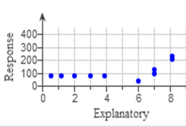
Non-linear Relationship
The data points do not have a linear relationship because they do not lie mainly on a straight line.


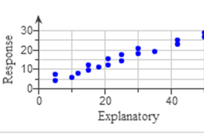
Positive Linear Relationship
The data points have a linear relationship because they lie mainly on a straight line.
However, the slope is positive.
This implies generally that as the predictor variable increases, the response variable increases.
This shows an increasing trend, which means that the value of the correlation coefficient will be positive.


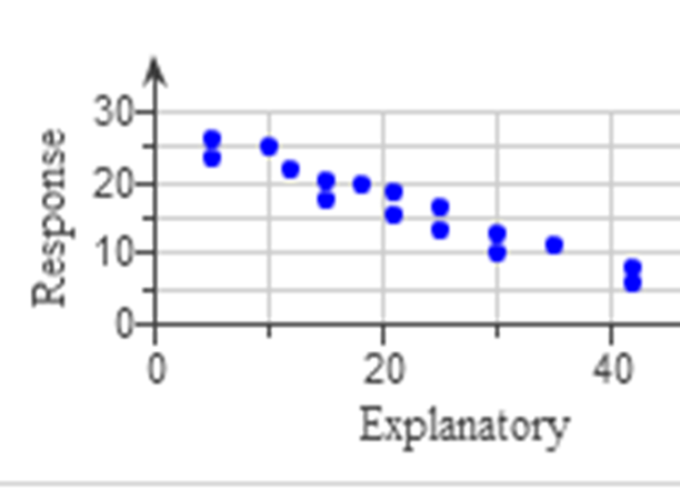
Negative Linear Relationship
The data points have a linear relationship because they lie mainly on a straight line.
However, the slope is negative.
This implies generally that as the predictor variable increases, the response variable decreases.
This shows a decreasing trend, which means that the value of the correlation coefficient will be negative.

Pearson Correlation Coefficient

(1.) The Pearson Correlation Coefficient, also known as the Product Moment Correlation Coefficient, also simply known as the Correlation Coefficient is a number that measures the strength of the linear association between two numerical variables.

(2.) It is denoted by r

(3.) It is a number between −1 and 1
This implies that: −1 ≤ r ≤ 1

(4.) It makes sense only if the trend is linear and the variables are numerical.

(5.) If the value of the correlation coefficient is positive, then the trend is positive.
If the value of the correlation coefficient is negative, then the trend is negative.

(6.) When computing the correlation coefficient for a pair of data sets, changing the order of the variables has no effect on the correlation coefficient.
In other words, the value of r when x is interchanged with y or y is interchanged with x

(7.) The correlation coefficient remains the same when adding a constant.

(8.) The correlation coefficient remains the same when multiplying by a positive constant.

NOTE: A correlation coefficient based on an observational study can never be used to support a claim of cause and effect.
This is because it is based on an observational study rather than on a designed experiment.

Coefficient of Determination

(1.) The Coefficient of Determination measures how much of the variation in the response variable is explained by the explanatory variable.

(2.) It is the square of the correlation coefficient, often called r-squared

(3.) It is denoted by r² or R²

(4.) It is between 0% and 100%.
A value of 0% indicates no linear relationship between the variables. Hence, the regression line does not predict the observations well.
A value of 100% indicates a strong linear relationship. Hence, the regression line perfectly predicts the observations.

Least-Squares Regression Line

(1.) The Least-Squares Regression Line also known as Linear Regression Equation or Line of Best Fit is a tool used for making predictions about future observed values.
In other words, we use it to predict a value of y, given the value of x.

(2.) It is also a useful way of summarizing a linear relationship.
Regression models are only useful for linear associations.

(3.) The word, predicted is often written in front of the y-variable in the equation of the regression line to emphasize that the line consists of the predicted y-values, rather than the actual y-values.

(4.) The name, least-squares line derives from the fact that it is chosen so that the sum of the squares of the differences between the observed y-values and the predicted y-values is as small as possible.

(5.) The intercept of a regression line gives the value of the predicted mean y-value when the x-value is 0.

(6.) Outliers have a big effect on the regression line because the regression line is a line of means.
An influential point is an outlier whose presence or absence has a big effect on the regression analysis.
If the data have one or more influential points, it is recommended to perform the regression analysis with and without these points, and comment on the differences.
Regression analysis should be performed with and without the influential points, to determine whether the influential points have an effect.

(7.) In the least-squares regression model, y_i = β₁x_i + β₀ + ε_i,
ε_i is a random error term with mean = 0, and
standard deviation σ_εi = σ

(8.) Regression towards the mean occurs when values for the predictor variable that are far from the mean lead to values of the response variable that are closer to the mean.
The farther the predictor variable is from the mean, the closer the response variable is to the mean.
The farther, x is from the mean, the closer y is to the mean.

NOTE: Extrapolation is defined as using the regression line to make predictions beyond the range of x-values in the data.
Because we develop the regression line using only the points in the data, extrapolation should not be used.

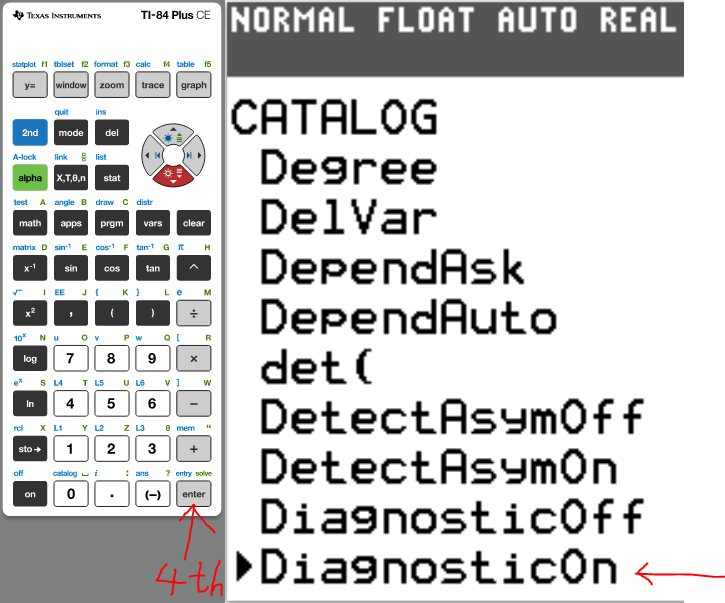
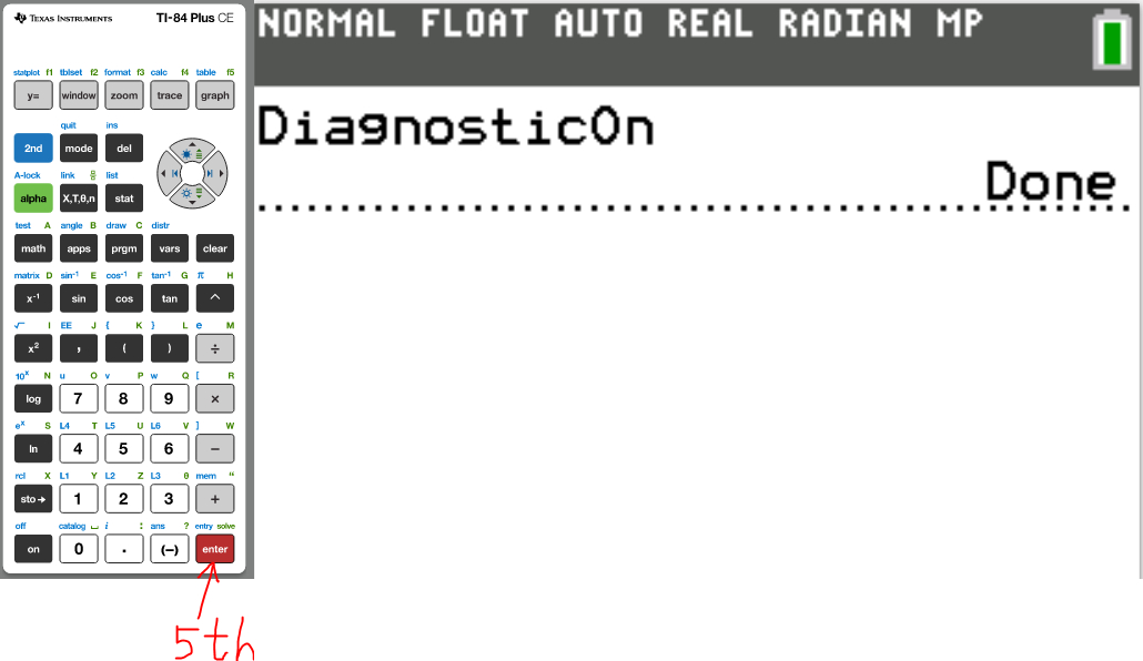
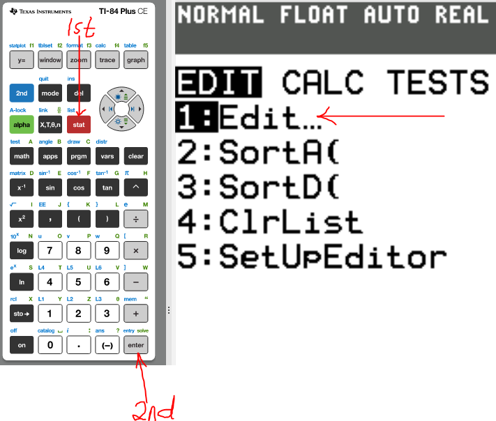
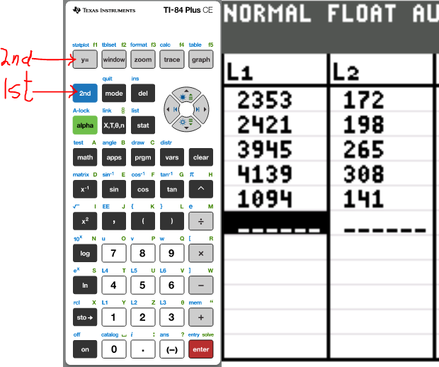
TI (Texas Instruments) Calculators

Set up the Calculator
The first thing we need to do is to turn Diagonstic On

(1.)

(2.)

(3.)

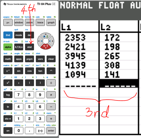
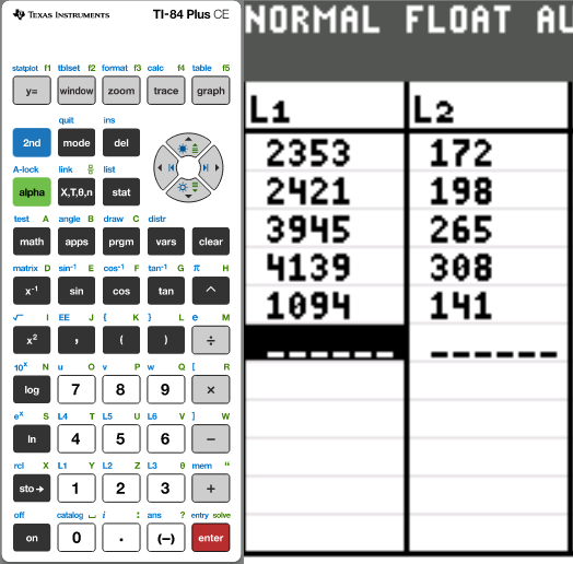
Example 1: The distance (in kilometers) and price (in dollars) for one-way airline tickets from San Francisco to several cities are shown in the table.

Destination	Distance (km)	Price ($)
Dallas Kansas City Baltimore New York City Seattle	2353 2421 3945 4139 1094	172 198 265 308 141

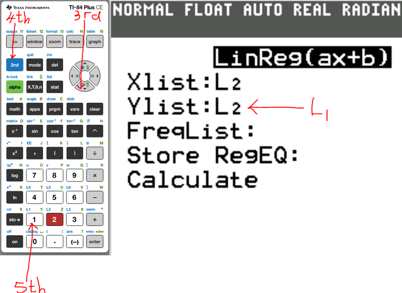
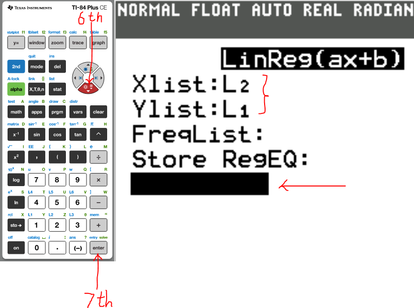
(a.) Determine the correlation coefficient for these data using a computer or statistical calculator.
Use distance as the x-variable and price as the y-variable.

(1.)

(2.)

(3.)

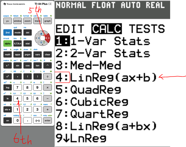
(4.)

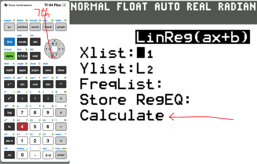
(5.)

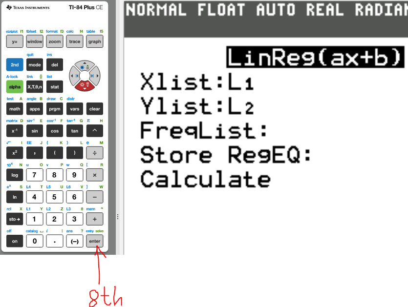
(6.)

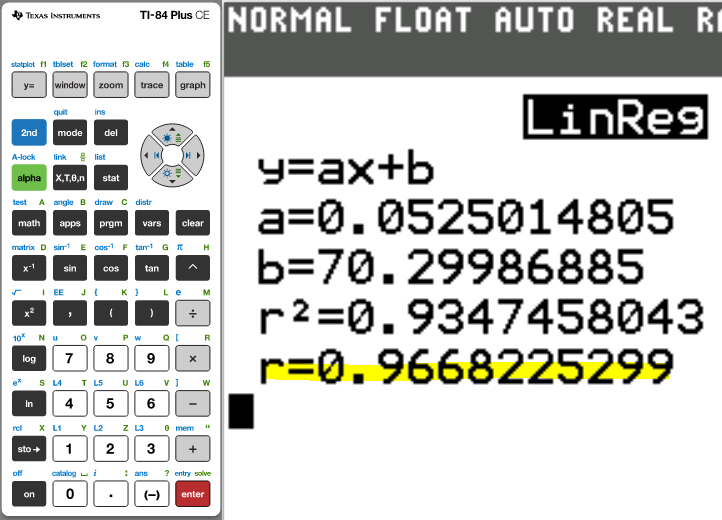
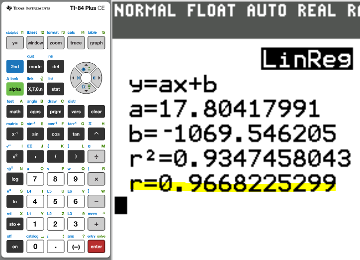
The correlation coefficient, r = 0.9668225299

(b.) Recalculate the correlation coefficient for these data using price as the x-variable and distance as the y-variable.
What effect does this have on the correlation coefficient?

(7.)

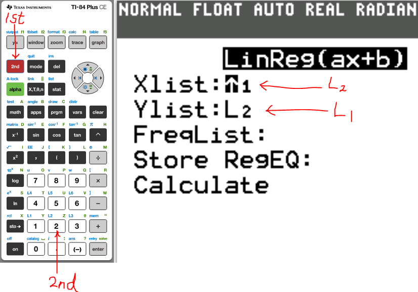
(8.)

(9.)

(10.)

The correlation coefficient, r = 0.9668225299
The correlation coefficient remains the same when the order of the variables is changed.

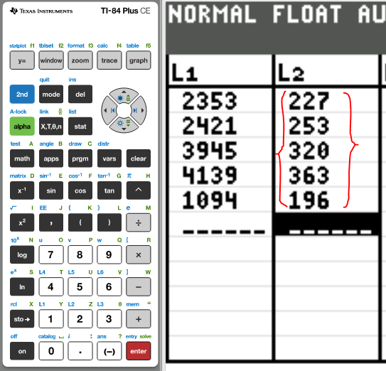
(c.) Suppose a $55 security fee was added to the price of each ticket.
What effect would this have on the correlation coefficient?

Destination	Distance (km)	Price ($)
Dallas Kansas City Baltimore New York City Seattle	2353 2421 3945 4139 1094	172 + 55 = 227 198 + 55 = 253 265 + 55 = 320 308 + 55 = 363 141 + 55 = 196

(11.)

(12.)

(13.)

The correlation coefficient, r = 0.9668225299
The correlation coefficient remains the same when adding a constant.

(d.) Suppose the airline held an incredible sale, where travelers got a round-trip ticket for the price of a one-way ticket.
This means that the distances would be doubled while the ticket price remained the same.
What effect would this have on the correlation coefficient?

Destination	Distance (km)	Price ($)
Dallas Kansas City Baltimore New York City Seattle	2353(2) = 4706 2421(2) = 4842 3945(2) = 7890 4139(2) = 8278 1094(2) = 2188	172 198 265 308 141

(14.)

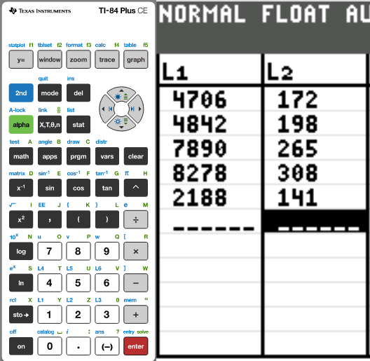
(15.)

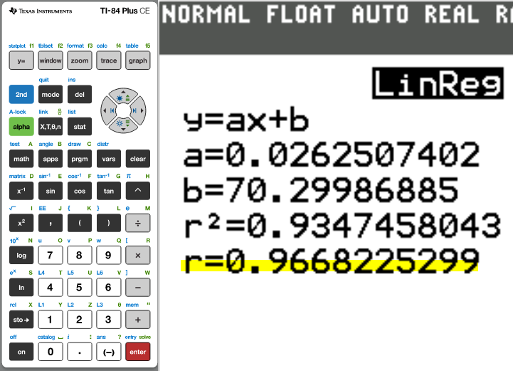
The correlation coefficient, r = 0.9668225299
The correlation coefficient remains the same when multiplying by a positive constant.

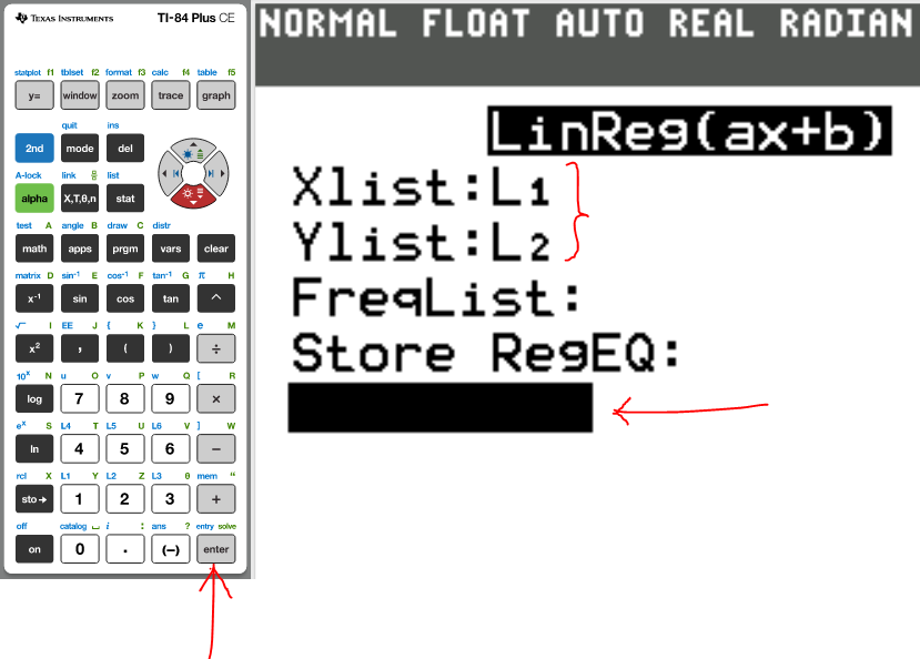
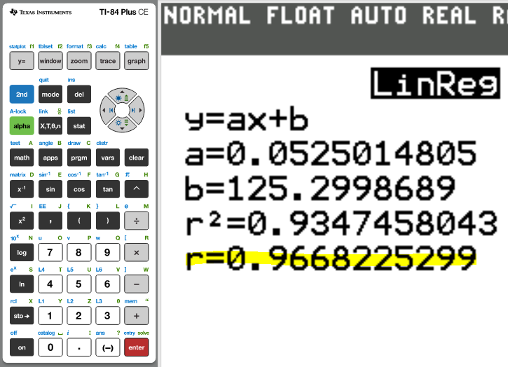
(e.) Using the initial dataset, write the equation of the least-squares line.
Linear Regression Equation


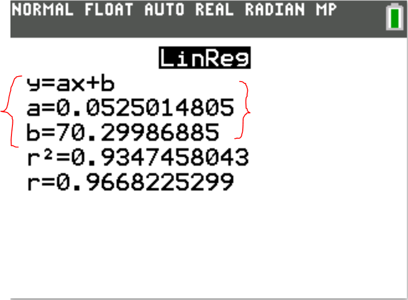
$ \hat{y} = b_{1}x + b_0 \\[3ex] \hat{y} = ax + b \\[3ex] \hat{y} = 0.0525014805x + 70.29986885 \\[3ex] $ (f.) Using the initial dataset, what is the coefficient of determination?
The coefficient of determination, r² = 0.9347458043

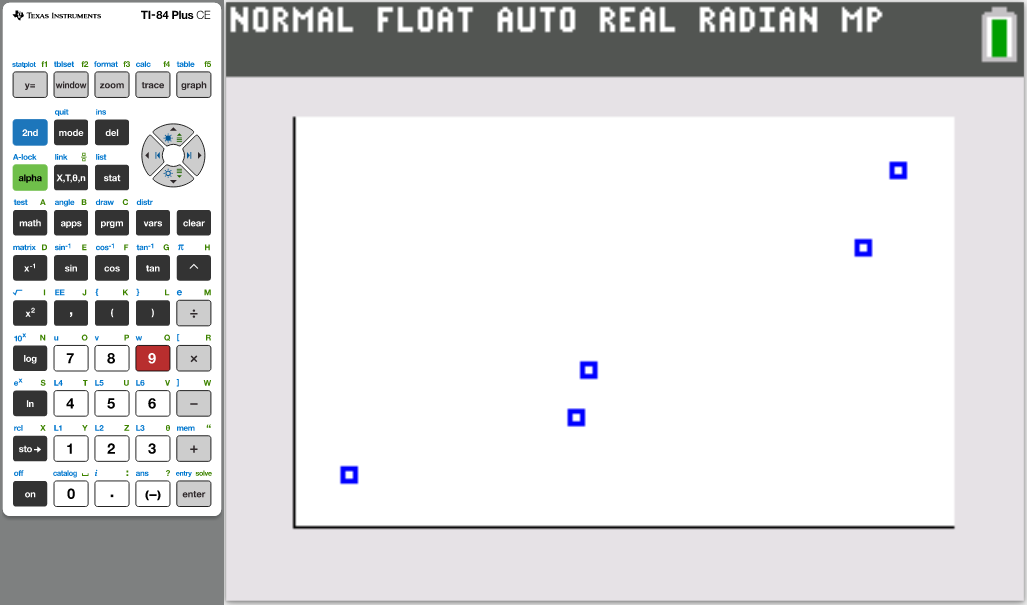
(g.) Draw the scatter diagram of the initial data.

(16.)

(17.)

(18.)

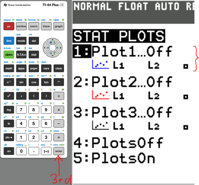
(19.)

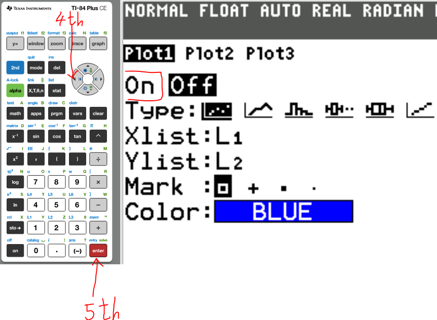
(20.)

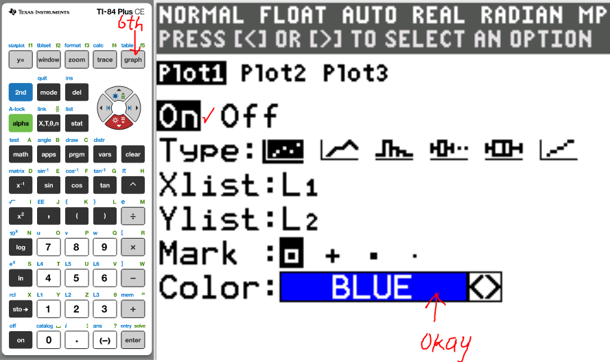
(21.)

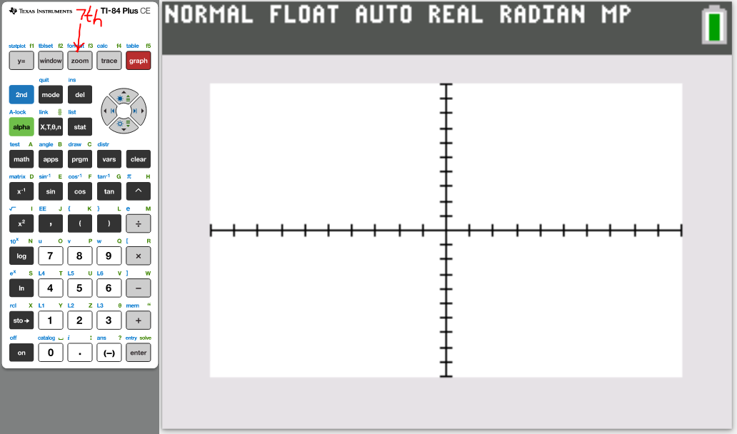
(22.)

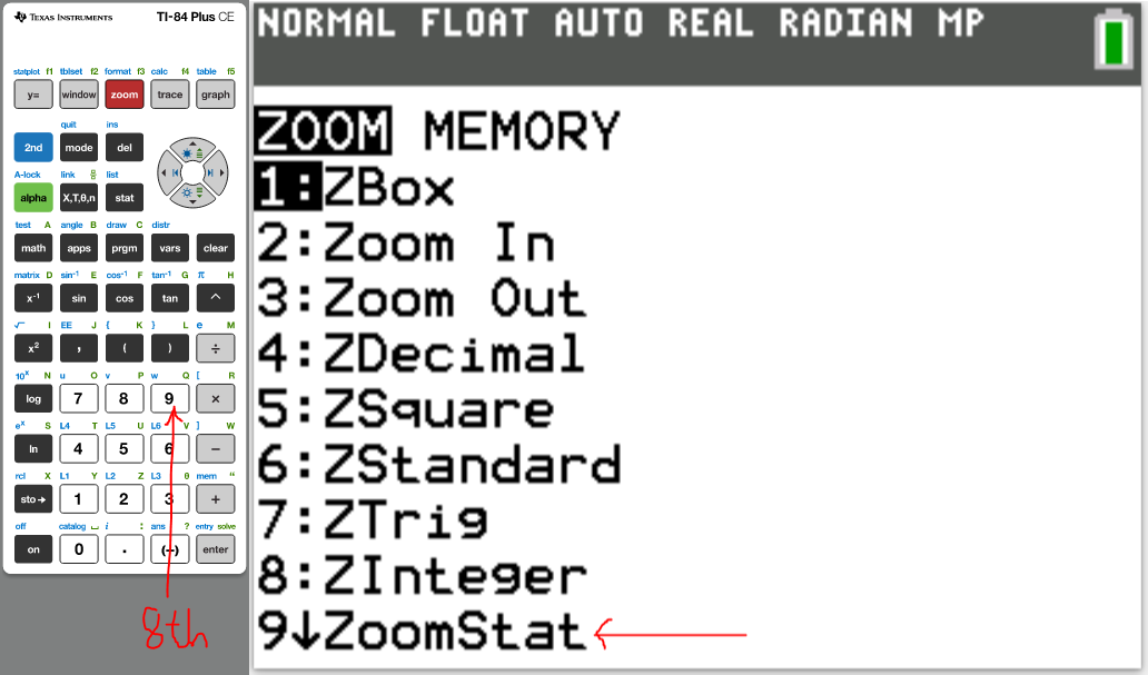
(23.)

Tables

References

Chukwuemeka, S.D (2033, January 10). Samuel Chukwuemeka Tutorials - Math, Science, and Technology. Retrieved from https://www.samuelchukwuemeka.com

Anderson, A. S., & Loeser, R. F. (2010, February). Why is Osteoarthritis an Age-Related Disease? Retrieved September 27, 2017, from https://www.ncbi.nlm.nih.gov/pmc/articles/PMC2818253/

Anderson, N. B. (1970, January 01). Race/Ethnicity, Socioeconomic Status, and Health. Retrieved September 27, 2017, from https://www.ncbi.nlm.nih.gov/books/NBK25526/

Black, Ken. (2012). Business Statistics for Contemporary Decision Making (7th ed.). New Jersey: Wiley

Gould, R., & Ryan, C. (2016). Introductory Statistics: Exploring the world through data (2nd ed.). Boston: Pearson

Gould, R., Wong, R., & Ryan, C. N. (2020). Introductory Statistics: Exploring the world through data (3rd ed.). Pearson.

Kozak, Kathryn. (2015). Statistics Using Technology (2nd ed.).

Nguyen, N. T., Nguyen, X. M., Lane, J., & Wang, P. (2011, March). Relationship between obesity and diabetes in a US adult population: findings from the National Health and Nutrition Examination Survey, 1999-2006. Retrieved September 27, 2017, from https://www.ncbi.nlm.nih.gov/pubmed/21128002

OpenStax, Introductory Statistics.OpenStax CNX. Sep 28, 2016. Retrieved from https://cnx.org/contents/30189442-6998-4686-ac05-ed152b91b9de@18.12

Smoking facts and evidence. (2017, June 26). Retrieved September 27, 2017, from http://www.cancerresearchuk.org/about-cancer/causes-of-cancer/smoking-and-cancer/smoking-facts-and-evidence#smoking_facts0

Sullivan, M., & Barnett, R. (2013). Statistics: Informed decisions using data with an introduction to mathematics of finance (2nd custom ed.). Boston: Pearson Learning Solutions.

Triola, M. F. (2015). Elementary Statistics using the TI-83/84 Plus Calculator (5th ed.). Boston: Pearson

Weiss, Neil A. (2015). Elementary Statistics (9th ed.). Boston: Pearson

Spearman Ranked Correlation Table. (n.d.). http://webspace.ship.edu/pgmarr/geo441/tables/spearman%20ranked%20correlation%20table.pdf

Elementary, Intermediate Tests and High School Regents Examinations : OSA : NYSED. (2019). Nysedregents.org. https://www.nysedregents.org/

GCSE Exam Past Papers: Revision World. Retrieved April 6, 2020, from https://revisionworld.com/gcse-revision/gcse-exam-past-papers

HSC exam papers | NSW Education Standards. (2019). Nsw.edu.au. https://educationstandards.nsw.edu.au/wps/portal/nesa/11-12/resources/hsc-exam-papers

NSC Examinations. (n.d.). www.education.gov.za. https://www.education.gov.za/Curriculum/NationalSeniorCertificate(NSC)Examinations.aspx

West African Examinations Council (WAEC). Retrieved May 30, 2020, from https://waeconline.org.ng/e-learning/Mathematics/mathsmain.html

D. (n.d.). Health Information for Your Health Needs. Retrieved September 27, 2017, from http://healthymedinfo.blogspot.com/2012/09/fever-and-headache-causes-and-treatment.html

(n.d.). Retrieved September 27, 2017, from http://web.cn.edu/kwheeler/logic_causation.html