If there is one prayer that you should pray/sing every day and every hour, it is the LORD's prayer (Our FATHER in Heaven prayer)
It is the most powerful prayer. A pure heart, a clean mind, and a clear conscience is necessary for it. - Samuel Dominic Chukwuemeka

For in GOD we live, and move, and have our being. - Acts 17:28

The Joy of a Teacher is the Success of his Students. - Samuel Dominic Chukwuemeka

Solved Examples and Applications of Correlation and Regression

Prerequisite: Descriptive Statistics

Calculators:
(1.) Vertical Data Entry: Correlation and Regression Calculators (Vertical Data Entry)
(2.) Horizontal Data Entry: Correlation and Regression Calculators (Horizontal Data Entry)

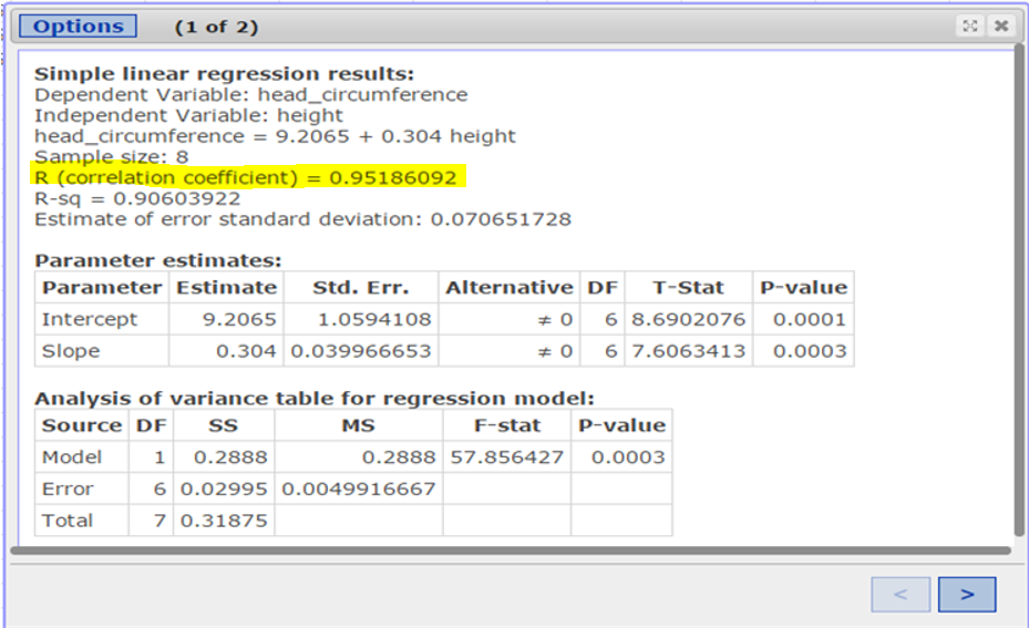
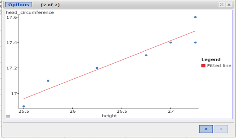
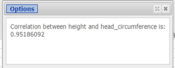
Technology: Pearson Statcrunch software

Tables Used:
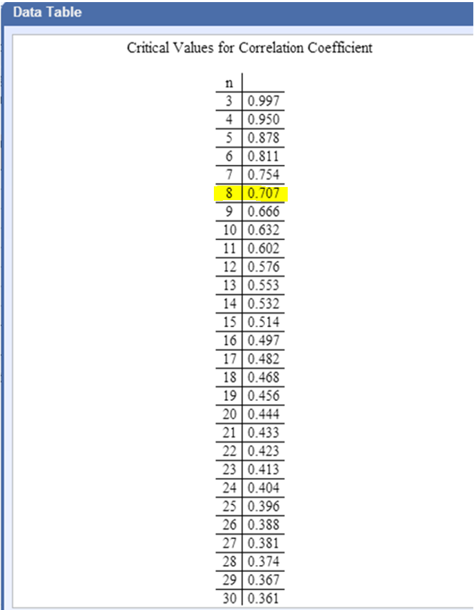
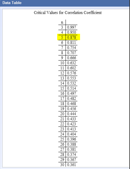
(1.) Based on Sample Size: Critical Values of the Pearson Correlation Coefficient
(2.) Based on Degrees of Freedom: Critical Values of the Pearson Correlation Coefficient
(3.) Based on Sample Size: Critical Values of the Spearman's Rank Correlation Coefficient

For ACT Students
The ACT is a timed exam...60 questions for 60 minutes
This implies that you have to solve each question in one minute.
Some questions will typically take less than a minute a solve.
Some questions will typically take more than a minute to solve.
The goal is to maximize your time. You use the time saved on those questions you solved in less than a minute, to solve the questions that will take more than a minute.
So, you should try to solve each question correctly and timely.
So, it is not just solving a question correctly, but solving it correctly on time.
Please ensure you attempt all ACT questions.
There is no negative penalty for any wrong answer.

For WASSCE Students
Any question labeled WASCCE is a question for the WASCCE General Mathematics
Any question labeled WASSCE-FM is a question for the WASSCE Further Mathematics/Elective Mathematics

For NSC Students
For the Questions:
Any space included in a number indicates a comma used to separate digits...separating multiples of three digits from behind.
Any comma included in a number indicates a decimal point.
For the Solutions:
Decimals are used appropriately rather than commas
Commas are used to separate digits appropriately.

Solve all questions.
Show all work.

Please Note:
(1.) For applicable questions, if the level of significance is not given, use 5%

(2.) Unless otherwise specified, do not round intermediate calculations.
However, if you must round intermediate calculations because of long decimal digits; then round those intermediate calculations to at least three (three or more) decimal places more than the number of decimal places to round the final answer.
For example: if the question asks you to round the final answer to three decimal places but did not specify how you should round intermediate calculations; then round the intermediate calculations to at least six decimal places.

(3.) Unless specified otherwise:
There are at least two formulas for calculating the Pearson's correlation coefficient.
For some questions, I shall use the First Formula.
For other questions, I shall use the Second Formula.
If you wish to see examples of how both formulas are used, please review all questions that asked for the determination of the correlation coefficient (or Pearson's correlation coefficient).

(1.) The scatterplot shows the median starting salaries and the median mid-career salaries for graduates at a selection of colleges. $$ Mid-Career = -17,092 + 2.067\;Start\;Med $$ Number 1

(a.) Identify the independent variable and the dependent variable.

(b.) Why is median salary used instead of the mean?

(c.) Using the graph, estimate the median mid-career salary for a median starting salary of $40000 (Round to the nearest dollar as needed)

(d.) Use the equation to predict the median mid-career salary for a median starting salary of $40000 (Round to the nearest dollar as needed)

(a.) The independent variable is the median starting salary.
The dependent variable is the median mid-career salary.

(b.) The median salary is used instead of the mean because the distribution of salaries is usually skewed. The median is a better measure of center for skewed distributions.

(c.) Using the graph, the median mid-career salary for a median starting salary of $40000 is about $\dfrac{50 + 75}{2} = \dfrac{125}{2}$ = $62.50 thousand ≈ $63000

$ (d.) \\[3ex] Mid-Career = -17,092 + 2.067\;Start\;Med \\[3ex] Mid-Career = -17092 + 2.067(40000) \\[3ex] Mid-Career = -17092 + 82680 \\[3ex] Mid-Career = 65588 \\[3ex] Mid-Career = \$65588 $

(2.) The distance (in kilometers) and price (in dollars) for one-way airline tickets from San Francisco to several cities are shown in the table.

Destination	Distance (km)	Price ($)
Dallas Kansas City Baltimore New York City Seattle	2353 2421 3945 4139 1094	172 198 265 308 141

(a.) Determine the correlation coefficient for these data using a computer or statistical calculator.
Use distance as the x-variable and price as the y-variable.

(b.) Recalculate the correlation coefficient for these data using price as the x-variable and distance as the y-variable.
What effect does this have on the correlation coefficient?

(c.) Suppose a $55 security fee was added to the price of each ticket.
What effect would this have on the correlation coefficient?

(d.) Suppose the airline held an incredible sale, where travelers got a round-trip ticket for the price of a one-way ticket.
This means that the distances would be doubled while the ticket price remained the same.
What effect would this have on the correlation coefficient?

The solution to this question is: here (in the home page)

(3.) In the game of baseball, the on-base percentage, x is the proportion of time a player reaches a base.
It is the best predictor of the winning percentage, y
For a certain baseball season, x and y are related by the regression equation: $\hat{y} = 2.92x - 0.4871$

(a.) What is the slope? Interpret the slope.

(b.) For this baseball season, the lowest on-base percentage was 0.318 and the highest on-base percentage was 0.358
Does it make sense to interpret the y-intercept?

(c.) Would it be a good idea to use this model to predict the winning percentage of a team whose on-base percentage was 0.240?

(d.) A certain team had an on-base percentage of 0.322 and a winning percentage of 0.544
Compute the residual.
Round to four decimal places as needed.

(e.) Interpret the residual.

(a.) The slope is 2.92 percentage.
For each percentage point increase in the on-base percentage, the winning percentage will increase by 2.92 percentage points, on average.

(b.) No, it would not make sense to interpret the y-intercept because it is outside the scope of the model.
Recall: To determine the y-intercept, we set $x = 0$ and solve for $y$
Lowest on-base percentage = 0.318
Highest on-base percentage = 0.358
0 does not lie between 0.318 and 0.358
It is outside the scope of the model.

(c.) No, it would not a good idea to use this model to predict the winning percentage because it is outside the scope of the model.
Lowest on-base percentage = 0.318
Highest on-base percentage = 0.358
0.240 does not lie between 0.318 and 0.358
It is outside the scope of the model.

(d.)

$ Observed\;\;x = 0.322 \\[3ex] Predicted\;\;y = \hat{y} = 2.92x - 0.4871 \\[3ex] \hat{y} = 2.92(0.322) - 0.4871 \\[3ex] \hat{y} = 0.94024 - 0.4871 \\[3ex] \hat{y} = 0.45314 \\[3ex] Observed\;\;y = 0.544 \\[3ex] Residual = Observed\;\;y - Predicted\;\;y \\[3ex] Residual = y - \hat{y} \\[3ex] Residual = 0.544 - 0.45314 \\[3ex] Residual = 0.09086 \\[3ex] Residual \approx 0.0909 \\[3ex] $ (e.)
The residual value of 0.0909 is positive.
This indicates that the winning percentage of the team is above average for teams with an on-base percentage of 0.322

Recall:
If the residual is positive, then the observed $y$ is greater than the predited $y$
Therefore the observed $y$ is above average for the observed $x$

If the residual is negative, then the observed $y$ is less than the predited $y$
Therefore the observed $y$ is below average for the observed $x$

If the residual is zero, then the observed $y$ is equal to the predicted $y$

(4.) The scatterplot shows the heights of mothers and daughters. $$ Daughter = 21.12 + 0.669\;Mother $$ Number 4

(a.) Identify the independent variable and the dependent variable.

(b.) Using the graph, approximate the predicted height of the daughter of a mother who is 55 inches (4 feet 7 inches) tall. (Round to the nearest inch as needed).

(c.) Use the equation to determine the predicted height of the daughter of a mother who is 55 inches (4 feet 7 inches) tall. (Round to two decimal places as needed).

(d.) What is the slope? Interpret the slope.

(a.) The independent variable is the mother's height.
The dependent variable is the daughter's height.

(b.) Using the graph, the approximate height of the daughter of a mother who is 55 inches (4 feet 7 inches) tall is about 58 inches.

$ (c.) \\[3ex] Daughter = 21.12 + 0.669\;Mother \\[3ex] Daughter = 21.12 + 0.669(55) \\[3ex] Daughter = 21.12 + 36.795 \\[3ex] Daughter = 57.915 \\[3ex] $ The daughter is about 57.92 inches tall.

(d.) The slope is 0.669 inch.
For each additional inch in the mother's height, the average daughter's height increases by about 0.669 inch.

(5.) The scatterplot shows the median weekly earnings (by quarter) for men and women in a country for the years from 2005 through 2017.
The correlation is 0.983

Number 5

(a.) Use the scatterplot to estimate the median weekly income for women in a quarter in which the median pay for men is about $750 (Round to the nearest dollar as needed).

(b.) Use the regression equation shown above the graph to get a more precise estimate of the median pay for women in a quarter in which the median pay for men is $750 (Round to the nearest cent as needed).

(c.) What is the slope of the regression equation?
Interpret the slope of the regression equation.

(d.) What is the y-intercept of the regression equation?
Interpret the y-intercept of the regression equation, or explain why it would be inappropriate to do so.

(a.) Based on the scatterplot, the median weekly income for women in a quarter in which the median pay for men is about $750 is about $600

$ (b.) \\[3ex] Predicted\;\;Women = -54.88 + 0.878\;Men \\[3ex] = -54.88 + 0.878(750) \\[3ex] = -54.88 + 650.5 \\[3ex] = 603.62 \\[3ex] $ The estimate of the median pay for women in a quarter in which the median pay for men is $750 is $603.62

(c.) The slope of the regression equation is 0.878
Each additional dollar in men's pay is associated with an increase of $0.878, on average, in the women's pay.

(d.) The y-intercept is −54.88
It is not appropriate to interpret the y-intercept since it does not make sense to have a median men's weekly pay of $0

(6.) A sociology class teacher gave a midterm exam and a final exam.
Assume that the association between midterm and final scores is linear.
The summary statistics are shown below.

	Mean	Standard deviation
Midterm	75	8
Final	75	8

The linear correlation coefficient is 0.75
The sample size is 30.

(a.) Find and report the equation of the regression line to predict the final exam score from the midterm score.

(b.) For a student who gets 54 on the midterm, predict the final exam score.
Round to the nearest integer as needed.

(c.) Explain why your answer in (b.) should be higher than 54.

(d.) Consider a student who gets a 100 on the midterm.
Without doing any calculations, state whether the predicted score on the final exam would be higher, lower, or the same as 100.

To predict the final exam score from the midterm score implies that:
y = final exam score
x = midterm score

$ \bar{x} = 75 \\[3ex] \bar{y} = 75 \\[3ex] s_x = 8 \\[3ex] s_y = 8 \\[3ex] r = 0.75 \\[3ex] (a.) \\[3ex] b_1 = r * \dfrac{s_y}{s_x} \\[5ex] = 0.75 * \dfrac{8}{8} \\[5ex] = 0.75 \\[5ex] b_0 = \bar{y} - b_1\bar{x} \\[3ex] = 75 - 0.75(75) \\[3ex] = 75 - 56.25 \\[3ex] = 18.75 \\[3ex] Least-squares\;\;regression\;\;line:\;\; \hat{y} = b_1x + b_0 \\[3ex] \hat{y} = 0.75x + 18.75 \\[3ex] Predicted\;\;Final\;\;Grade = 0.75(Midterm\;\;Grade) + 18.75 \\[5ex] (b.) \\[3ex] Midterm\;\;Grade = 54 \\[3ex] Predicted\;\;Final\;\;Grade = 0.75(Midterm\;\;Grade) + 18.75 \\[3ex] = 0.75(54) + 18.75 \\[3ex] = 40.5 + 18.75 \\[3ex] = 59.25 \\[3ex] \approx 59 \\[5ex] $ Regression towards the mean occurs when values for the predictor variable that are far from the mean lead to values of the response variable that are closer to the mean.

(c.) The student's final score should be higher than his or her midterm score because of regression toward the mean: predictor variables far from the mean tend to produce response variables closer to the mean.
The farther the predictor variable is from the mean, the closer the response variable is to the mean.
The farther, x is from the mean, the closer y is to the mean.

(d.) The predicted score on the final exam would be lower than 100 because of regression toward the mean.

(12.) Given that:

$ \bar{x} = 1.833 \\[3ex] s_x = 2.228602 \\[3ex] \bar{y} = 5.067 \\[3ex] s_y = 1.5253415 \\[3ex] r = -0.9021256 \\[3ex] $ Determine the least-squares regression line.
Round to four decimal places as needed.

$ b_1 = r * \dfrac{s_y}{s_x} \\[5ex] = -0.9021256 * \dfrac{1.5253415}{2.228602} \\[5ex] = -\dfrac{1.376049616}{2.228602} \\[5ex] = -0.6174496908 \\[3ex] \approx -0.6175 \\[5ex] b_0 = \bar{y} - b_1\bar{x} \\[3ex] = 5.067 - (-0.6174496908)(1.833) \\[3ex] = 5.067 + 1.131785283 \\[3ex] = 6.198785283 \\[3ex] b_0 \approx 6.1988 \\[3ex] Least-squares\;\;regression\;\;line:\;\; \hat{y} = b_1x + b_0 \\[3ex] \hat{y} = -0.6175x + 6.1988 $

(15.) GCSE Competitors in the Paris Figure Skating competition in the Winter Olympics perform twice.
The competitors are awarded points each time.
The table shows the points awarded to the top 10 pairs in the 2018 Winter Olympics.

Names of competitors	Performance 1	Performance 2
Savchenko & Massot	76.59	159.31
Sui & Han	82.39	153.08
Duhamel & Radford	76.81	153.33
Tarasova & Morozov	81.68	143.25
James & Cipress	75.34	143.19
Marchei & Hotarek	74.50	142.09
Zabiiako & Enbert	74.34	138.53
Yu & Zhang	75.58	128.52
Seguin & Bilodeau	67.52	136.50
Della Monica & Guarise	74.00	128.74

(a.) Calculate the value of Spearman's Rank Correlation Coefficient between the points scored in the two performances.

Use $r_s = 1 - \dfrac{6\Sigma d^2}{n(n^2 - 1)} \;\;\;and\;\;\; \Sigma d^2 = 50$

(b.) Interpret your answer to part (a.) in context.

Depending on time:
Ask students to verify that the sum of the square of the differences is fifty
In other words, ask students to verify that $\Sigma d^2 = 50$
Verify each step of their calculations with the calculators.

(a.)
$ n = 10 \\[3ex] \Sigma d^2 = 50 \\[3ex] r_s = 1 - \dfrac{6\Sigma d^2}{n(n^2 - 1)} \\[5ex] = 1 - \dfrac{6 * 50}{10(10^2 - 1)} \\[5ex] = 1 - \dfrac{300}{10(100 - 1)} \\[5ex] = 1 - \dfrac{300}{10(99)} \\[5ex] = 1 - \dfrac{300}{990} \\[5ex] = 1 - 0.303030303 \\[3ex] = 0.696969697 \\[3ex] $ (b.)
There is a positive correlation between the awarded points in the two performances by the set of competitors.
Competitors who did well in the first performance tend to do well in the second performance.

(16.) Divine Mercy Pediatrics wants to determine if there is a relationship between a child's height and the head circumference.
Eight patients were randomly selected, and the table below shows their height and head circumference measurements.

Height (inches)	$27$	$25.75$	$26.75$	$25.5$	$27.25$	$26.25$	$26.25$	$27.25$
Head Circumference (inches)	$17.4$	$17.1$	$17.3$	$16.9$	$17.6$	$17.2$	$17.2$	$17.4$

(a.) Determine with reasons, the response variable and the explanatory variable.
(b.) Draw a scatter diagram.
(c.) Compute the linear correlation coefficient.
For this question, round intermediate calculations to four decimal places as needed.
Round the final answer to three decimal places as needed.
(d.) Interpret your result.

(a.) The response variable is the head circumference
The explanatory variable is the height
This is because the head circumference depends on the height on the child, not the other way around.
The response variable, $y-variable$ is the dependent variable (it depends on $x$)
The explanatory or predictor variable, $x-variable$ is the independent variable.

(b.) The scatter diagram is as shown:
Number 16(b.)

(c.) First Formula is used.

$x$	$x - \bar{x}$	$(x - \bar{x})^2$	$y$	$y - \bar{y}$	$(y - \bar{y})^2$
$27$	$0.5$	$0.25$	$17.4$	$0.1375$	$0.0189$
$25.75$	$-0.75$	$0.5625$	$17.1$	$-0.1625$	$0.0264$
$26.75$	$0.25$	$0.0625$	$17.3$	$0.0375$	$0.0014$
$25.5$	$-1$	$1$	$16.9$	$-0.3625$	$0.1314$
$27.25$	$0.75$	$0.5625$	$17.6$	$0.3375$	$0.1139$
$26.25$	$-0.25$	$0.0625$	$17.2$	$-0.0625$	$0.0039$
$26.25$	$-0.25$	$0.0625$	$17.2$	$-0.0625$	$0.0039$
$27.25$	$0.75$	$0.5625$	$17.4$	$0.1375$	$0.0189$
$\Sigma x = 212$	$\Sigma (x - \bar{x})^2 = 3.125$		$\Sigma y = 138.1$	$\Sigma (y - \bar{y})^2 = 0.3187$

$ \bar{x} = \dfrac{\Sigma x}{n} \\[5ex] = \dfrac{212}{8} \\[5ex] = 26.5 \\[3ex] \bar{y} = \dfrac{\Sigma y}{n} \\[5ex] = \dfrac{138.1}{8} \\[5ex] = 17.2625 \\[3ex] s_{x} = \sqrt{\dfrac{\Sigma(x - \bar{x})^2}{n - 1}} \\[5ex] = \sqrt{\dfrac{3.125}{8 - 1}} \\[5ex] = \sqrt{\dfrac{3.125}{7}} \\[5ex] = \sqrt{0.4464285714} \\[3ex] = 0.6681531048 \\[3ex] \approx 0.6682 \\[3ex] s_{y} = \sqrt{\dfrac{\Sigma(y - \bar{y})^2}{n - 1}} \\[5ex] = \sqrt{\dfrac{0.3187}{8 - 1}} \\[5ex] = \sqrt{\dfrac{0.3187}{7}} \\[5ex] = \sqrt{0.04552857143} \\[3ex] = 0.213374252 \\[3ex] \approx 0.2134 \\[3ex] $

$x$	$x - \bar{x}$	$\dfrac{x - \bar{x}}{s_x}$	$y$	$y - \bar{y}$	$\dfrac{y - \bar{y}}{s_y}$	$\left(\dfrac{x - \bar{x}}{s_x}\right)\left(\dfrac{y - \bar{y}}{s_y}\right)$
$27$	$0.5$	$0.7483$	$17.4$	$0.1375$	$0.6443$	$0.4822$
$25.75$	$-0.75$	$-1.1224$	$17.1$	$-0.1625$	$-0.7615$	$0.8547$
$26.75$	$0.25$	$0.3741$	$17.3$	$0.0375$	$0.1757$	$0.0657$
$25.5$	$-1$	$-1.4966$	$16.9$	$-0.3625$	$-1.6987$	$2.5423$
$27.25$	$0.75$	$1.1224$	$17.6$	$0.3375$	$1.5815$	$1.7751$
$26.25$	$-0.25$	$-0.3741$	$17.2$	$-0.0625$	$-0.2929$	$0.1096$
$26.25$	$-0.25$	$-0.3741$	$17.2$	$-0.0625$	$-0.2929$	$0.1096$
$27.25$	$0.75$	$1.1224$	$17.4$	$0.1375$	$0.6443$	$0.7232$
$\Sigma \left(\dfrac{x - \bar{x}}{s_x}\right)\left(\dfrac{y - \bar{y}}{s_y}\right) = 6.6624$

$ r = \dfrac{\Sigma\left(\dfrac{x - \bar{x}}{s_x}\right)\left(\dfrac{y - \bar{y}}{s_y}\right)}{n - 1} \\[7ex] = \dfrac{6.6624}{8 - 1} \\[5ex] = \dfrac{6.6624}{7} \\[5ex] = 0.952 \\[3ex] $ We can also compute the correlation coefficient by using the Pearson Statcrunch software
Number 16(c.)(i)

(d.)

Absolute value of the correlation coefficient = |0.952| = 0.952
Critical Value of the correlation coefficient for a sample size of 8 = 0.707
Because:
(1.) the absolute value of the correlation coefficient is greater than the critical value of the correlation coefficient for a sample size of 8:
and
(2.) the correlation coeffient is positive:
there is a positive linear correlation between a child's height and the head circumference.

(17.) WASSCE-FM In a research to determine the relationship between performance of students in an entrance examination and subsequent school performance, the results of ten randomly selected students were obtained as follows:

Students	$A$	$B$	$C$	$D$	$E$	$F$	$G$	$H$	$I$	$J$
Performance in Entrance Examination	$11$	$12$	$8$	$13$	$6$	$15$	$10$	$14$	$17$	$16$
School Performance	$5$	$10$	$9$	$7$	$4$	$8$	$6$	$14$	$11$	$12$

(a.) Calculate the Spearman's rank correlation coefficient.
(b.) What would be the researcher's conclusion from the result in (a.)

Performance in Entrance Examination, $X$	$11$	$12$	$8$	$13$	$6$	$15$	$10$	$14$	$17$	$16$
Rank $X$	$4$	$5$	$2$	$6$	$1$	$8$	$3$	$7$	$10$	$9$

School Performance, $Y$	$5$	$10$	$9$	$7$	$4$	$8$	$6$	$14$	$11$	$12$
Rank $Y$	$2$	$7$	$6$	$4$	$1$	$5$	$3$	$10$	$8$	$9$

Performance in Entrance Examination, $X$	School Performance, $Y$	$R_X$	$R_Y$	$d = R_X - R_Y$	$d^2$
$11$	$5$	$4$	$2$	$2$	$4$
$12$	$10$	$5$	$7$	$-2$	$4$
$8$	$9$	$2$	$6$	$-4$	$16$
$13$	$7$	$6$	$4$	$2$	$4$
$6$	$4$	$1$	$1$	$0$	$0$
$15$	$8$	$8$	$5$	$3$	$9$
$10$	$6$	$3$	$3$	$0$	$0$
$14$	$14$	$7$	$10$	$-3$	$9$
$17$	$11$	$10$	$8$	$2$	$4$
$16$	$12$	$9$	$9$	$0$	$0$
				$\Sigma d^2 = 50$

$ (a.) \\[3ex] n = 10 \\[3ex] n^2 = 10^2 = 100 \\[3ex] n^2 - 1 = 100 - 1 = 99 \\[3ex] \rho = 1 - \dfrac{6\Sigma d^2}{n(n^2 - 1)} \\[5ex] = 1 - \dfrac{6(50)}{10(99)} \\[5ex] = 1 - \dfrac{300}{990} \\[5ex] = 1 - 0.303030303 \\[3ex] = 0.696969697 \\[3ex] $ (b.) Based on the result from (a.)
Because the Spearman's rank correlation coefficient is positive, there is a positive correlation between performance in entrance examination and school performance and vice versa.
This implies that a student who performs well in entrance examination also tends to perform well in school.
Similarly, a student who perfoms well in school tends to perform well in the entrance examination.

(18.) For the data set below:
(a.) Draw the scatter diagram
(b.) Compute the correlation coefficient.
(c.) Interpret the correlation coefficient.

$x$	$7$	$6$	$6$	$7$	$9$
$y$	$3$	$7$	$6$	$9$	$5$

(a.) The scatter diagram is drawn as follows:
Number 18a

(b.) Second Formula is used.

$x$	$y$	$x^2$	$y^2$	$xy$
$7$	$3$	$7^2 = 49$	$3^2 = 9$	$7 * 3 = 21$
$6$	$7$	$6^2 = 36$	$7^2 = 49$	$6 * 7 = 42$
$6$	$6$	$6^2 = 36$	$6^2 = 36$	$6 * 6 = 36$
$7$	$9$	$7^2 = 49$	$9^2 = 81$	$7 * 9 = 63$
$9$	$5$	$9^2 = 81$	$5^2 = 25$	$9 * 5 = 45$
$\Sigma x = 35$	$\Sigma y = 30$	$\Sigma x^2 = 251$	$\Sigma y^2 = 200$	$\Sigma xy = 207$

$ n = 5 \\[3ex] r = \dfrac{n(\Sigma xy) - (\Sigma x)(\Sigma y)}{\sqrt{n(\Sigma x^2) - (\Sigma x)^2} * \sqrt{n(\Sigma y^2) - (\Sigma y)^2}} \\[5ex] = \dfrac{5(207) - (35)(30)}{\sqrt{5(251) - (35)^2} * \sqrt{5(200) - (30)^2}} \\[5ex] = \dfrac{1035 - 1050}{\sqrt{1255 - 1225} * \sqrt{1000 - 900}} \\[5ex] = \dfrac{-15}{\sqrt{30} * \sqrt{100}} \\[5ex] = \dfrac{-15}{10(5.477225575)} \\[5ex] = \dfrac{-15}{54.77225575} \\[5ex] = -0.2738612788 \\[3ex] \approx -0.274 \\[3ex] $ (c.)
Number 18ci

Because the absolute value of the correlation coefficient: $0.274$ is not greater than the critical value for the sample size of 5: $0.878$, no linear relation exists between $x$ and $y$

(19.) NSC The wind speed (in km per hour) and temperature (in °C) for a certain town were recorded at 16:00 for a period of 10 days.
The information is shown in the table below.

WIND SPEED IN km/h ($x$)	2	6	15	20	25	17	11	24	13	22
TEMPERATURE IN °C ($y$)	28	26	22	22	16	20	24	19	26	19

(19.1) Determine the equation of the least squares regression line for the data.
(19.2) Predict the temperature at 16:00 if, on a certain day, the wind speed of this town was 9 km per hour.
(19.3) Interpret the value of b in the context of the data.

(19.1)

$x$	$x - \bar{x}$	$(x - \bar{x})^2$	$\dfrac{x - \bar{x}}{s_x}$
$2$	$-13.5$	$182.25$	$-1.765045216$
$6$	$-9.5$	$90.25$	$-1.242068856$
$15$	$-0.5$	$0.25$	$-0.065372045$
$20$	$4.5$	$20.25$	$0.588348405$
$25$	$9.5$	$90.25$	$1.242068856$
$17$	$1.5$	$2.25$	$0.196116135$
$11$	$-4.5$	$20.25$	$-0.588348405$
$24$	$8.5$	$72.25$	$1.111324766$
$13$	$-2.5$	$6.25$	$-0.326860225$
$22$	$6.5$	$42.25$	$0.849836586$
$ \Sigma x = 155 \\[3ex] n = 10 \\[3ex] \bar{x} = \dfrac{\Sigma x}{n} \\[5ex] \bar{x} = \dfrac{155}{10} \\[5ex] \bar{x} = 15.5 $		$ \Sigma (x - \bar{x})^2 = 526.5 \\[5ex] s_x = \sqrt{\dfrac{\Sigma (x - \bar{x})^2}{n - 1}} \\[5ex] = \sqrt{\dfrac{526.5}{9}} \\[5ex] = \sqrt{58.5} \\[3ex] = 7.64852927 $

$y$	$y - \bar{y}$	$(y - \bar{y})^2$	$\dfrac{y - \bar{y}}{s_y}$
$28$	$5.8$	$33.64$	$1.528434202$
$26$	$3.8$	$14.44$	$1.001387926$
$22$	$-0.2$	$0.04$	$-0.052704628$
$22$	$-0.2$	$0.04$	$-0.052704628$
$16$	$-6.2$	$38.44$	$-1.633843458$
$20$	$-2.2$	$4.84$	$-0.579750904$
$24$	$1.8$	$3.24$	$0.474341649$
$19$	$-3.2$	$10.24$	$-0.843274043$
$26$	$3.8$	$14.44$	$1.001387926$
$19$	$-3.2$	$10.24$	$-0.843274043$
$ \Sigma y = 222 \\[3ex] n = 10 \\[3ex] \bar{y} = \dfrac{\Sigma y}{n} \\[5ex] \bar{y} = \dfrac{222}{10} \\[5ex] \bar{y} = 22.2 $		$ \Sigma (y - \bar{y})^2 = 129.6 \\[5ex] s_y = \sqrt{\dfrac{\Sigma (y - \bar{y})^2}{n - 1}} \\[5ex] = \sqrt{\dfrac{129.6}{9}} \\[5ex] = \sqrt{14.4} \\[3ex] = 3.794733192 $

$\left(\dfrac{x - \bar{x}}{s_x}\right) \left(\dfrac{y - \bar{y}}{s_y}\right)$
$-2.697755477$
$-1.243792755$
$0.003445409$
$-0.031008684$
$-2.029346074$
$-0.113698507$
$-0.279078153$
$-0.937151328$
$-0.327313883$
$-0.716645133$
$\Sigma \left(\dfrac{x - \bar{x}}{s_x}\right) \left(\dfrac{y - \bar{y}}{s_y}\right) = -8.372344585$

$ r = \dfrac{\Sigma\left(\dfrac{x - \bar{x}}{s_x}\right)\left(\dfrac{y - \bar{y}}{s_y}\right)}{n - 1} \\[5ex] = -\dfrac{8.372344585}{10 - 1} \\[5ex] = -\dfrac{8.372344585}{9} \\[5ex] = -0.9302605094 \\[3ex] b_1 = r * \dfrac{s_y}{s_x} \\[5ex] = -0.9302605094 * \dfrac{3.794733192}{7.64852927} \\[5ex] = -\dfrac{3.530090432}{7.64852927} \\[5ex] = -0.4615384615 \\[3ex] b_0 = \bar{y} - b_1\bar{x} \\[3ex] = 22.2 - (-0.4615384615)(15.5) \\[3ex] = 22.2 - (-7.153846154) \\[3ex] = 22.2 + 7.153846154 \\[3ex] = 29.35384615 \\[3ex] Least-squares\;\;regression\;\;line: \\[3ex] \hat{y} = b_1 x + b_0 \\[3ex] \hat{y} = -0.4615384615x + 29.35384615 \\[5ex] (19.2) \\[3ex] x = 9\;\;km/h \\[3ex] \hat{y} = -0.4615384615(9) + 29.35384615 \\[3ex] \hat{y} = -0.4615384615x + 29.35384615 \\[3ex] \hat{y} = -4.153846154 + 29.35384615 \\[3ex] \hat{y} = 25.2^\circ C \\[3ex] $ (19.3)
$b = b_1 = slope = -0.4615384615$
The negative slope implies that as the wind speed, $x$ increases, the temperature, $y$ decreases.
The negative value of the slope implies that on average; if the wind speed increases by 1 km/h, the temperature decreases by 0.4615384615 °C

(20.) HSC Mathematics Standard/Advanced 2 A cricket is an insect. The male cricket produces a chirping sound.
A scientist wants to explore the relationship between the temperature in degrees Celsius and the number of cricket chirps heard in a 15-second time interval.
Once a day for 20 days, the scientist collects data. Based on the 20 data points, the scientist provides the information below.
A box-plot of the temperature data is shown.

The mean temperature in the dataset is 0.525°C below the median temperature in the dataset.
A total of 684 chirps was counted when collecting the 20 data points.
The scientist fits a least-squares regression line using the data $(x, y)$, where $x$ is the temperature in degrees Celsius and $y$ is the number of chirps heard in a 15-second time interval.
The equation of the line is $y = -10.6063 + bx$,
where $b$ is the slope of the regression line.
The least-squares regression line passes through the point $(\bar{x}, \bar{y})$ where $\bar{x}$ is the sample mean of the temperature data and $\bar{y}$ is the sample mean of the chirp data.
Calculate the number of chirps expected in a 15-second interval when the temperature is 19° Celsius.
Give your answer correct to the nearest whole number.

$x$ = temperature in degrees Celsius
$y$ = number of chirps in a 15-second time interval

Based on the five-number summary in the box-plot:

$ Median:\;\; \tilde{x} = 22^\circ C \\[3ex] Mean:\;\;\bar{x} = 22 - 0.525 = 21.475^\circ C \\[3ex] \underline{Number\;\;of\;\;chirps:\;\;y} \\[3ex] \Sigma y = 684 \\[3ex] n = 20 \\[3ex] \bar{y} = \dfrac{\Sigma y}{n} \\[5ex] \bar{y} = \dfrac{684}{20} \\[5ex] \bar{y} = 34.2 \\[3ex] \underline{Equation\;\;of\;\;the\;\;line} \\[3ex] y = -10.6063 + bx...eqn.(1) \\[3ex] Passes\;\;through\;\;(\bar{x},\bar{y}) \\[3ex] Passes\;\;through\;\;(21.475, 34.2) \\[3ex] \implies \\[3ex] x_1 = 21.475 \\[3ex] y_1 = 34.2\;chirps \\[3ex] \underline{Equation\;\;of\;\;a\;\;straight\;\;line\;\;passing\;\;through\;\;a\;\;point} \\[3ex] y - y_1 = b(x - x_1) \\[3ex] y - 34.2 = b(x - 21.475) \\[3ex] y - 34.2 = bx - 21.475b \\[3ex] y = bx - 21.475b + 34.2 ...eqn.(2) \\[3ex] Equate\;\;eqn.(1)\;\;and\;\;eqn.(2) \\[3ex] y = y \\[3ex] \implies \\[3ex] -10.6063 + bx = bx - 21.475b + 34.2 \\[3ex] 21.475b = bx + 34.2 + 10.6063 - bx \\[3ex] 21.475b = 44.8063 \\[3ex] b = \dfrac{44.8063}{21.475} \\[5ex] b = 2.086440047 \\[3ex] Substitute\;\;for\;\;b\;\;in\;\;eqn.(1) \\[3ex] \therefore y = -10.6063 + 2.086440047x \\[3ex] when\;\;x = 19^\circ C \\[3ex] y = -10.6063 + 2.086440047(19) \\[3ex] y = -10.6063 + 39.64236088 \\[3ex] y = 29.03606088 \\[3ex] y \approx 29\;\;chirps $

Top